Friday, 29 May 2009

JVisualVM and Clojure

JVisualVM is a Java Virtual machine monitoring tool that allows you to see a live view of the Java memory, cpu and threads that are currently active. In this post, I'll look at how easy it is to profile Clojure code using JVisualVM.

First step is to get jvisualvm installed. If you've got a recent JDK then it's already available in the bin directory of the JDK install. If not, then upgrade to the latest JDK here. Once installed, fire it up and you should see the following.

jvirtualvm startup screen

The left hand side shows the applications you can connect to. You should see a VisualVM instance that allows you to monitor the VisualVM itself. Very meta. The local applications will include all locally running Java applications. Since Clojure itself is a Java application we can fire up a REPL and use that to profile code.

Firstly we'll look at garbage collection by using the memory profiler. People often associate immutable data structures (such as Clojure's) with poor performance since every time we modifying a data structure we are actually creating a completely new structure (in reality that's not quite true, structure that is unchanged is often shared). Using JVisualVM we can profile how fast the JVM can allocate objects. Let's use a really simple example which sums up the numbers 1 to 100K. Without JVirtualVM this takes 40ms. In those 40 seconds we create at least 100K objects.


user> (time (reduce + (range 100000))
"Elapsed time: 40.677795 msecs"
4999950000


If we instrument this we can see that 165K java.lang.Integer objects are created together with 35K java.lang.Long objects. In this example then we're creating roughly 4 million objects per second! Pretty impressive (I realize this is totally non scientific, I'm just aiming to get a feel for the numbers!).
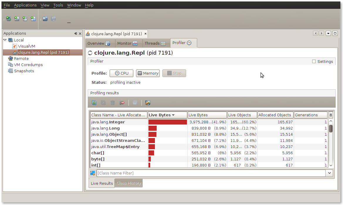
REPL profile

Another area in which you can apply JVisualVM is looking for optimizations and monitoring threads. In one of my previous posts, I looked at Mandlebrot fractal generation. We can use jvisualvm to understand the performance characteristics of the application. The only interesting part of the code for this experiment is shown below:


(defn calculate-pixels []
(let [pixels (range 0 (* *width* *height*))]
(pmap (fn [p]
(let [row (rem p *width*) col (int (/ p *height*))]
(get-color (process-pixel (/ row (double *width*)) (/ col (double *height*))))))
pixels)))


Running this with a single-threaded map instead of pmap gives us the following CPU information.
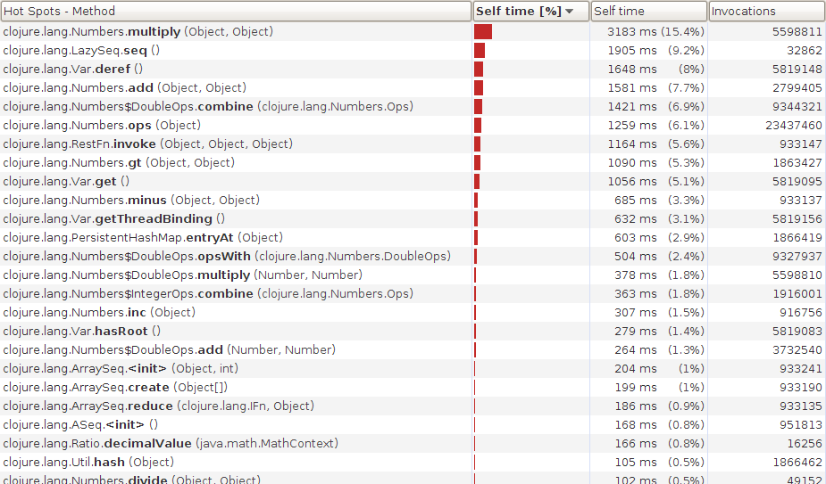
Single-threaded

The time is dominated by mathematical operations. This is what you'd expect. You'd expect (naively) if you used multiple threads you'd be able to speed things up since the operations on each pixel are independent. What happens if we switch to pmap?
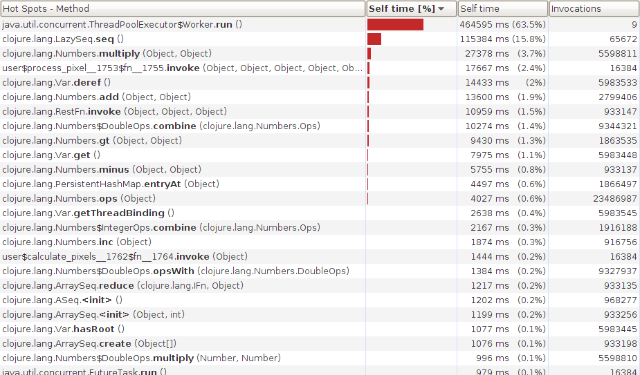
Using multiple threads

There's a big change. The time now is dominated by ThreadPoolExecutor$Worker which is taking up a huge percentage of the time. My guess is that we're context switching far too much - using jvisualvm we can get a view of what the threads were doing:
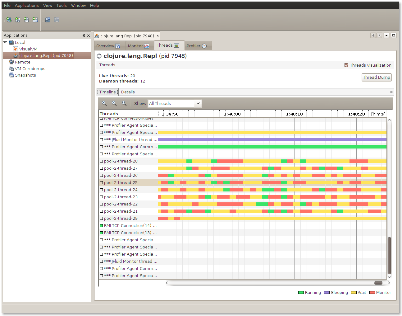
Lots of threads

The image shows that the threads spent a lot of time waiting and not a lot of time doing processing. Opportunities for simultaneous processing were few because of the time spent spawning off tiny amounts of work.

Let's partition off chunkier bits of works in an effort to make the CPU work harder for its money. In the function below I use partition to break the set of pixels to render into 16 discrete chunks (number chosen at random). We use pmap again but this time it's got chunker bits of work to do. doall is used to force the evaluation of the inner map.


(defn calculate-pixels-2 []
(let [n (* *width* *height*)
work (partition (/ n 16) (range 0 n))
result (pmap (fn [x]
(doall (map
(fn [p]
(let [row (rem p *width*) col (int (/ p *height*))]
(get-color (process-pixel (/ row (double *width*)) (/ col (double *height*))))))
x)))
work)]
(doall (apply concat result))))


The difference this makes is very visible. The graphic below shows two runs. Each time we can see that the threads are fully busy, not blocked and able to fully utilize the CPU. The worker threads are indicated at the bottom in the image below.
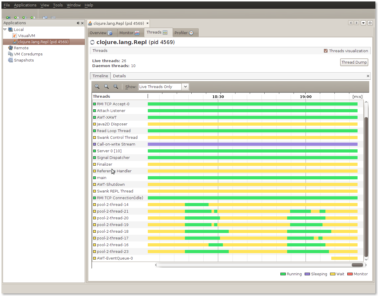
Full use of threads when using pmap

So using VisualVM helped quantify various improvements. Whilst premature optimization is the root of all evil, if you are going to optimize then it should be guided by a tool rather than your intuition (which if you are anything like me is more often than not crap).
Monday, 25 May 2009

Neural Networks and Clojure

Neural Networks (ANNs) attempt to "learn" by modelling the behaviour of neurons. Although neural networks sound cool, there is no magic behind them!

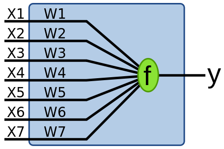
Invented in 1957, by Frank Rosenblatt, the single layer perceptron network is the simplest type of neural network. The single layer perceptron network is able to act as a binary classifier for any linearly separable data set.

Single Layer Perceptron graphic from Wikipedia

The SLP is nothing more than a collection of weights and an output value. The Clojure code below allows you to create a network (initially with zero weights) and get a result from the network given some weights and an input. Not very interesting.


(defn create-network
[out]
(repeat in 0))

(defn run-network
[input weights]
(if (pos? (reduce + (map * input weights))) 1 0))


The clever bit is adapting the weights so that the neural network learns. This process is known as training and is based on a set of data with known expectations. The learning algorithm for SLPs is shown below. Given an error (either 1 or -1 in this case), adjust the weights based on the size of the inputs. The learning-rate decides how much to vary the weights; too high and the algorithm won't converge, too low and it'll take forever to converge.


(def learning-rate 0.05)

(defn- update-weights
[weights inputs error]
(map
(fn [weight input] (+ weight (* learning-rate error input)))
weights inputs))


Finally, we can put this all together with a simple training function. Given a series of samples and the expected values, repeatedly update the weights until the training set is empty.


(defn train
([samples expecteds] (train samples expecteds (create-network (count (first samples)))))
([samples expecteds weights]
(if (empty? samples)
weights
(let [sample (first samples)
expected (first expecteds)
actual (run-network sample weights)
error (- expected actual)]
(recur (rest samples) (rest expecteds) (update-weights weights sample error))))))


So we have our network now. How can we use it? Firstly, let's define a couple of data sets both linearly separable and not. jiggle adds some random noise to each sample. Note the cool # syntax for a short function definition (I hadn't seen it before).


(defn jiggle [data]
(map (fn [x] (+ x (- (rand 0.05) 0.025))) data))

(def linearly-separable-test-data
[(concat
(take 100 (repeatedly #(jiggle [0 1 0])))
(take 100 (repeatedly #(jiggle [1 0 0]))))
(concat
(repeat 100 0)
(repeat 100 1))])

(def xor-test-data
[(concat
(take 100 (repeatedly #(jiggle [0 1])))
(take 100 (repeatedly #(jiggle [1 0])))
(take 100 (repeatedly #(jiggle [0 0])))
(take 100 (repeatedly #(jiggle [1 1]))))
(concat
(repeat 100 1)
(repeat 100 1)
(repeat 100 0)
(repeat 100 0))])


If we run these in the REPL we can see that the results are perfect for the linearly separable data.


> (apply train ls-test-data)
(0.04982859491606148 -0.0011851610388172009 -4.431771581539448E-4)

> (run-network [0 1 0] (apply train ls-test-data))
0

> (run-network [1 0 0] (apply train ls-test-data))
1


However, for the non-linearly separable they are completely wrong:


> (apply train xor-test-data)
(-0.02626745010362212 -0.028550312499346104)

> (run-network [1 1] (apply train xor-test-data))
0

> (run-network [0 1] (apply train xor-test-data))
0

> (run-network [1 0] (apply train xor-test-data))
0

> (run-network [0 0] (apply train xor-test-data))
0


The neural network algorithm shown here is really just a gradient descent optimization that only works for linearly separable data. Instead of calculating the solution in an iterative manner, we could have just arrived at an optimal solution in one go.

More complicated networks, such as the multi-layer perceptron network have more classification power and can work for non linearly separable data. I'll look at them next time!

Friday, 22 May 2009

How to improve coding

Reddit has gone downhill (it's almost as bad as Digg), but there are still some insightful comments. Take this answer regarding how to become better at programming:


  • "Buy lots of cans of paint and start doodling. Only artsy types can be true hackers.

  • Learn everything there is to know about manhole covers. This shows you have vital knowledge outside of programming.

  • Study to be an architect, find patterns everywhere and name them. Write a programming book about it and bask in the fame.

  • Become proficient in programming languages you will never use seriously. Only the best can afford to waste time so.

  • Keep up with the fads of the day while holding on to religious tenets of the past. You will be flexible yet dependable.

  • Read a book about motorcycle maintenance and see its deep connections to programming. You will seem mysterious and wise.

  • Know deep in your heart that you're in the top 10% of all programmers. Superiority is a state of mind.

  • When you once get the hang of programming, you know everything. There is no elephant, only tree trunks all alike."


  • This touches on most of the memes regarding improving as a programmer that I've seen. Hackers and Painters, crazy interview questions, read SICP, extreme programming and the 10x gap in performance.